Simulasi Motor BLDC dengan Python

Dengan mengetahui karakteristik dari Motor BLDC, kita dapat membuat simulasinya dengan variabel-variabel yang kita inginkan. Hal ini sangat berguna untuk mengetahui respon dari BLDC motor jika mengubah beberapa variabel tanpa perlu melakukan trial and error pada perangkat kerasnya. Oleh karena itu, penulis mencoba malakukan simulasi Motor BLDC dengan Python.

Kalau belum mengetahui apa itu motor BLDC, bisa membaca terlebih dahulu artikelnya disini. Kemudian untuk mengetahui lebih dalam, tentang Motor BLDC beserta kontrollernya bisa mengakses pada tulisan Stefan Baldursson disini. Simulasi dengan Python menjadi pilihan karena cukup mudah digunakan dan banyak referensinya.

Simulasi ini dapat diakses pada repository ini. Program tersebut merupakan hasil forked dari repo sebelumnya(dituliskan pada README repository) yang menggunakan Python 2.6, kemudian diupgrade sedikit pada repository ini dengan menggunakan Python3 (Penulis menggunakan Python 3.6). Selain itu simulasi juga memerlukan package numpy, dan scipy yang telah telah terpasang. Untuk cara memasangnya bisa dilihat disini.

Untuk melakukan simulasi bisa clone atau download reponya.

git clone https://github.com/zharfanw/open-bldc-pysim

Selanjutnya, jalan program sim_1.py

#
# Open-BLDC pysim - Open BrushLess DC Motor Controller python simulator
# Copyright (C) 2011 by Antoine Drouin <poinix@gmail.com>
# Copyright (C) 2011 by Piotr Esden-Tempski <piotr@esden.net>
#
# This program is free software; you can redistribute it and/or modify
# it under the terms of the GNU General Public License as published by
# the Free Software Foundation; either version 3 of the License, or
# (at your option) any later version.
#
# This program is distributed in the hope that it will be useful,
# but WITHOUT ANY WARRANTY; without even the implied warranty of
# MERCHANTABILITY or FITNESS FOR A PARTICULAR PURPOSE.  See the
# GNU General Public License for more details.
#
# You should have received a copy of the GNU General Public License
# along with this program.  If not, see <http://www.gnu.org/licenses/>.
#

import matplotlib
# matplotlib.use('MacOSX')
# matplotlib.use('GTKCairo')
import numpy as np
import pylab as pl
import matplotlib.pyplot as plt
from scipy import integrate
from scipy.signal import decimate

import misc_utils as mu
import dyn_model  as dm
import control    as ctl
import my_io      as mio
import my_plot    as mp



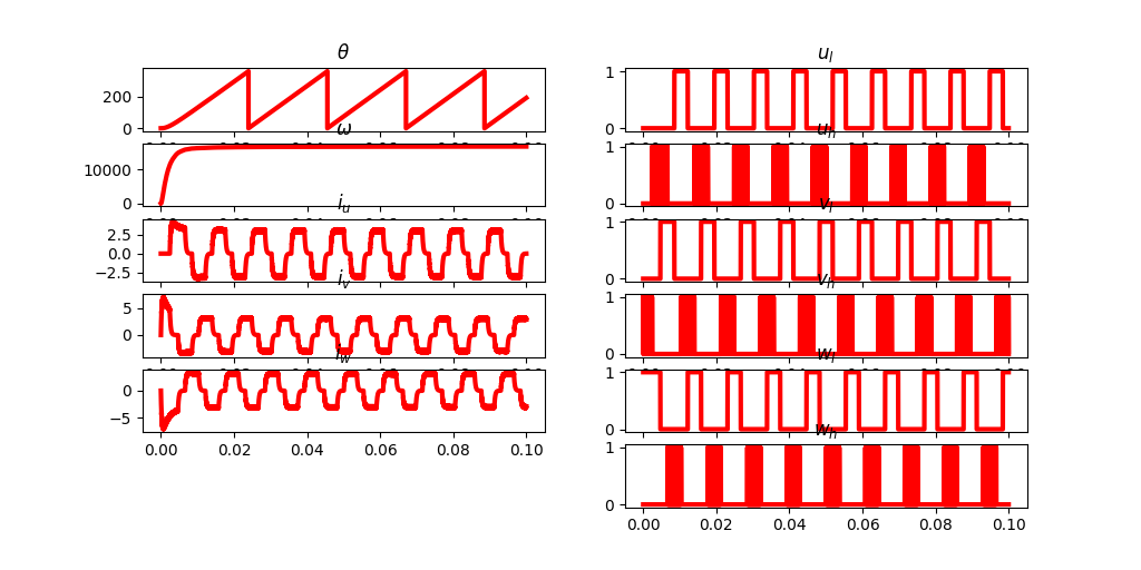
def display_state_and_command(time, X, U):

    titles_state = ['$\\theta$', '$\omega$', '$i_u$', '$i_v$', '$i_w$']
    titles_cmd = ['$u_l$', '$u_h$', '$v_l$', '$v_h$', '$w_l$', '$w_h$']
    for i in range(0, 2):
        plt.subplot(6, 2, 2*i+1)
        plt.plot(time,mu.deg_of_rad(X[:,i]), 'r', linewidth=3.0)
        plt.title(titles_state[i])
    for i in range(2, dm.sv_size):
        plt.subplot(6, 2, 2*i+1)
        plt.plot(time, X[:,i], 'r', linewidth=3.0)
        plt.title(titles_state[i])
    for i in range(0, 6):
        plt.subplot(6, 2, 2*i+2)
        plt.plot(time, U[:,i], 'r', linewidth=3.0)
        plt.title(titles_cmd[i])

def print_simulation_progress(count, steps):
        sim_perc_last = ((count-1)*100) / steps
        sim_perc = (count*100) / steps
        if (sim_perc_last != sim_perc):
            print ("{}%".format(sim_perc))

def drop_it(a, factor):
	new = []
	for n, x in enumerate(a):
		if ((n % factor) == 0):
			new.append(x)
	return np.array(new)

def compress(a, factor):
	return drop_it(a, factor)
	#return decimate(a, 8, n=8, axis=0)

def main():
#    t_psim, Y_psim =  mio.read_csv('bldc_startup_psim_1us_resolution.csv')
#    mp.plot_output(t_psim, Y_psim, '.')

    freq_sim = 1e6                              # simulation frequency
    compress_factor = 3
    time = pl.arange(0.0, 0.1, 1/freq_sim) # create time slice vector
    X = np.zeros((time.size, dm.sv_size))       # allocate state vector
    Xdebug = np.zeros((time.size, dm.dv_size))  # allocate debug data vector
    Y = np.zeros((time.size, dm.ov_size))       # allocate output vector
    U = np.zeros((time.size, dm.iv_size))       # allocate input vector
    X0 = [0, mu.rad_of_deg(0.1), 0, 0, 0]       #
    X[0,:] = X0
    W = [0, 1]
    for i in range(1,time.size):

        if i==1:
            Uim2 = np.zeros(dm.iv_size)
        else:
            Uim2 = U[i-2,:]

        Y[i-1,:] = dm.output(X[i-1,:], Uim2)                  # get the output for the last step
        U[i-1,:] = ctl.run(0, Y[i-1,:], time[i-1])            # run the controller for the last step
        tmp = integrate.odeint(dm.dyn, X[i-1,:], [time[i-1], time[i]], args=(U[i-1,:], W)) # integrate
        X[i,:] = tmp[1,:] # copy integration output to the current step
        X[i, dm.sv_theta] = mu.norm_angle( X[i, dm.sv_theta]) # normalize the angle in the state
        tmp, Xdebug[i,:] = dm.dyn_debug(X[i-1,:], time[i-1], U[i-1,:], W) # get debug data
        print_simulation_progress(i, time.size)

    Y[-1,:] = Y[-2,:]
    U[-1,:] = U[-2,:]

    if compress_factor > 1:
        time = compress(time, compress_factor)
        Y = compress(Y, compress_factor)
        X = compress(X, compress_factor)
        U = compress(U, compress_factor)
        Xdebug = compress(Xdebug, compress_factor)

    mp.plot_output(time, Y, '-')
#    pl.show()
    plt.figure(figsize=(10.24, 5.12))
    display_state_and_command(time, X, U)

    plt.figure(figsize=(10.24, 5.12))
    mp.plot_debug(time, Xdebug)

    pl.show()

if __name__ == "__main__":
    main()

dan hasilnya adalah sebagai berikut

Dengan adanya simulasi ini, semoga dapat bermanfaat.

Author colekmes

Saya seperti core of the core pada website ini :)